Probability for Machine learning

Probability is the basic we must know for Machine learning and to begin with I believe ‘Random Variable’ is the best to start with.

In this blog, you may notice few topics are just introduced and are not explained end to end, that’s because I am trying to cover topics that matter more in Machine learning perspective.

What is a Random Variable?

As per the definition by “Google” :

“A random variable is a variable whose value is unknown, or a function that assigns values to each of an experiment’s outcomes.”

Sounds Hard? Let me try to explain better.

What if I say, A random variable is any one possible outcome of the experiment that we are performing. For example: A Dice that have six sides {1,2,3,4,5,6} can get any of these 6 numbers when I roll it, in other words, I can say that ‘X’ is a random variable that can take any value from {1,2,3,4,5,6} when a dice is rolled. Please note that ‘X’ is a variable that can hold ‘1’ value its not an array or list.

Types of Random Variable

To make it simple there are two categories of a random variable

1. Discrete Random Variable
2. Continuous Random Variable

Discrete Random Variable

When you have a range very well defined and from that range there can be one outcome then it is a discrete random variable. What does that mean? Let’s go back to the dice example, the only and only possible outcomes are {1,2,3,4,5,6} and we can’t get 4.5 in our experiment of rolling one dice. Then X is a discrete random variable. Few more examples of discrete random variables are:

1. A bag full of balls
2. Levels of a game
3. Number of chocolates in a chocolate box.

Continuous Random Variable

When an event do not have a very well defined range, or in other words we can say, there is a dense range for e.g. [4,5] have a countibily infine range between 4 and 5, and from that range there can be one outcome then it is a continuous random variable.

What does that mean?  When you are trying to estimate/guess (not calculate) a height of person, then, can you be accurate to the 10 decimal places? Certainly, not. That means even if you are extremely close to say that person is nearly 162 cm, there is a chance of at least 10^th decimal place it is less or more, which means we do not have a straight forward range. This is an example of Continuous Random Variable Few more examples of Continuous random variable are:

1. Weight of entity
2. Speed of a vehicle
3. Timestamps

Permutations and Combinations for Probability

Probability and Permutations & Combinations go hand in hand, so we must take a quick look at the permutations & Combinations formula before we go ahead,

What is permutation and combinations?

If I am tossing a coin 3 times, then how many “combinations” of output I may get, let’s take a look:

As displayed above, for a simple coin, tossed 3 thrice, there are 8 combinations of output that are possible.

To be noted here, when we are trying to find all the possible outcomes then order of head and tails does matter and we can simply calculate this by using a logic

2 outcomes in each flip, so for three flips => 2*2*2 = 8 or simply 2³ 

Now suppose, I need to know out of total outcomes how may will have exactly 2 tails.

Then, each outcome comprises of 3 values ‘HHH’ for example and we want to know how many ways two tails can be arranged and how many ways 1 head can be arranged in this set of three values. We have a simple formula to calculate this

where n is the number of values in a set, r is the number desired output. For our example we have a set of three so n = 3 and we want to arrange 2 tails so r = 2.

 

Which results in 3 and we can verify the same using our toss chart.

For our current goal, we do not need to dive deep into Permutations & Combinations and knowing the formula and how to solve it would suffice. I will take this example forward to explain probability.

Probability:

The chance of an event to occur in the given number of trials is called probability.

By this I mean if I want my dice to throw 5 for me, then the chances I will get 5 are 1/6.

How? Total numbers of outcomes a die may have are 6 so my sample size is 6 {1,2,3,4,5,6} and I want just 1 number from it (my choice is 5, it could be ‘4’ or ‘3’ or any number within {1,2,3,4,5,6})

So, Probability = Desired outcome/ Total number of possible outcomes

It’s not always that straight forward and this is the most basic example I gave.

Lets go back to coin toss example and calculate the probability of getting exactly two tails when a coin is flipped thrice

As we have already saw from our calculations in permutaions & combinations sections we know that,

Total outcomes possible are 8 and out of which 3 times its possible to get exactly 2 tails.  So our probability would be 3/8.

Now lets look at few interesting concepts on which probability highly depends.

Independent, Dependent and Mutually Exclusive trials:

Suppose my problem statement says: “From a bag full of 5 blue and 6 red balls, what is the chance/probability of getting exactly blue ball in each of the 3 trails while drawing one ball at a time”

Dependent trials:

 

Dependent trials are the ones when the outcome of one trial impacts the probability of other trail.  In problem stated above, if, I am checking the color of the ball and not re-placing it back in bag, rather keeping it aside then the total number of balls are changing for each following trail and hence impacting their probabilities.

Independent trials:

If in each trial I am checking the color of the ball and putting it back in bag, then my total number of balls in bags remains same for each trail and probability of getting a blue ball will remain same in all the trails. So I can say, “The outcome of one trial is independent of the other trial”

Mutually Exclusive trials:

If I roll a die then, on one outcome I can’t get 2 values together. I can either get 1 or 2 or 3 etc. or all of them are mutually exclusive and have nothing to do with each other. Such events are Mutually exclusive events/trials.

Conditional Probability:

Another very important concept in probability is Conditional Probability, which is basically trying to find a probability of an event based on a condition given or assumed. Notation for Conditional Probability is as follows:

P (A|B): This should be read as, probability of event A; given that event B already happened.

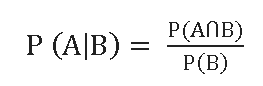                         provided P (B) >0

It is best to understand Conditional probability through example, so that we understamd the concept rather than learning definition.

Rolling a dice again: As we saw above, the sample size for a dice is {1,2,3,4,5,6} and probability of getting 3

Now if I say:

Given an odd number is rolled what is the probability of getting 3?

In this case our reduced sample size is {1,3,5} and probability of getting a 3 now

This probability we derived using basic probability logic, we can get the same using formula stated above

Entire sample size: {1,2,3,4,5,6}

Let getting 3 in entire sample size is Event A = {3}

and all odds is Event B = {1,3,5}

Then, probability of A and B both happening is  which is getting probability of A and B both happening in entire sample size and that just once that is ‘3’, so

And probability of event B in entire sample space.

Hence, by Conditional probability formula:

 This example is taken from Sir Jeremy Balka’s statistics lectures. Thanks to him for amazing content to grasp this concept with such ease.

Probability Distributions:

As the name suggests, it shows for an event how the probability is distributed for a certain range of values.

For both the types for random variables there are probability distributions:

1. Discrete Probability distributions
2. Random Probability distributions

Discrete Probability distributions

Probability distribution for a discrete random variable, as discrete random variables have jump in numbers and hence the probability distribution is represented by a histogram.

Discrete Probability distributions characterized into various kinds, few are listed as below.

1. Binomial Distribution: We apply Binomial distribution when we are trying to find the number of success in ‘N’ INDEPENDENT trails
2. Hyper-Geometric Distribution: We apply Hyper-Geometric distribution when we are trying to find the number of success in ‘N’ DEPENDENT trails
3. Geometric Distribution: This is used when we try for find the 1^st success in ‘N’ independent trials.
4. Negative Binomial Distribution: This is used when we try for find the n^th success in ‘N’ independent trials.

Continuous probability distributions:

Probability distribution for a continuous random variable, as continuous random variables have dense bunch of values e.g. within [4, 5] there is a big range of numbers (often called countably infinite) and hence the probability distribution is represented by a curve (Bell shaped curve).

Continuous Probability distributions characterized into various kinds, few are listed as below.

1. Normal distribution
2. Log-Normal distribution
3. Pareto distribution

Continuous probability distributions are extremly important in Machine learning and its unfair to put one-liners for them hence, I will discuss these in detail in another blog.

Naive Bayes Classifier in Machine Learning:

Now that we know probability and conditional probability, lets understand a very important machine learning algorithm Naive Bayes Classification Algorithm.